|
If you’ve ever seen the squiggly red line under a word and chosen the “Add to Dictionary”? That is the custom dictionary in Microsoft Office. All of those words are stored in a custom dictionary file on your computer’s hard drive. If you add a word to the dictionary but need to edit or remove it, you can. Also you can transfer the custom Office dictionary from one computer to another. To access the Custom Dictionary: In Word , go to File, Options, and then in the Proofing section you’ll see “Custom Dictionaries. Once in the Dictionary you can click on Edit Word List or view the path of where it is saved at on your computer. 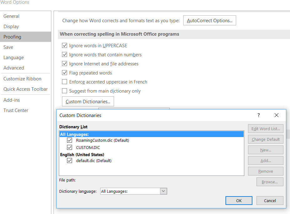
0 Comments
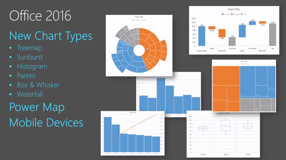
There are new chart types in Excel 2016, including Waterfall, Sunburst, Tree map, Funnel, Histogram, Pareto, and Box and Whisker. They can be used from programs like, Excel, Outlook, PowerPoint, and Word. Here are a few details:
 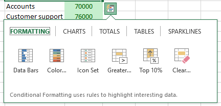 Here's how - there is a new feature in Excel 2013/2016 called Quick Analysis. Simply select a range of cells then click the icon that appears at the bottom right corner to reveal options like creating a quick formula, table, chart and more. This is one of the many new features in Excel - others include major enhancements to Charts, new Formulas, Flash Fill and more.
The Microsoft Excel SUMIFS function lets you specify multiple IF conditions within one formula and add together cells based on the conditions. It can be used to evaluate if multiple conditions are true do this, but if they are false do this. For example, you would use SUMIFS to sum the number of retailers in the country who (1) reside in a single zip code and (2) whose profits exceed a specific dollar value. Syntax: SUMIFS(sum_range, criteria_range1, criteria1, [criteria_range2, criteria2], ...) Sum Range is the range of cells you want to add together. The criteria range is the range(s) you want to evaluate with the criteria being the condition.  Excel, Outlook, PowerPoint, Word 2016 all have a new option on the Insert tab of the Ribbon – Icons. Once you open the Icons window, click on a category from the left-hand side. Once you find the Icon you want to use click Insert. You will have a Graphic Tools tab on the Ribbon with additional options for formatting the Icon. To learn more about this feature or other new Office 2016 options, attend one of our classes.
 The Microsoft Excel SUMIFS function lets you specify multiple IF conditions within one formula and add together cells based on the conditions. It can be used to evaluate if multiple conditions are true do this, but if they are false do this. For example, you would use SUMIFS to sum the number of retailers in the country who (1) reside in a single zip code and (2) whose profits exceed a specific dollar value. Syntax: SUMIFS(sum_range, criteria_range1, criteria1, [criteria_range2, criteria2], ...) Sum Range is the range of cells you want to add together. The criteria range is the range(s) you want to evaluate with the criteria being the condition.
 Excel has built-in lists of data that you can enter by using the fill handle. When you hesitate your mouse on the bottom right corner of the active cell, you will see a black t, this is the fill handle. The custom lists included with Excel are; days of the week, months and quarters. You can also use these custom lists to sort data and you can create your own custom lists. Here is an example of how to enter data from a custom list: Type in Monday then use the fill handle to drag down or across cells. As you move across cells it will fill in Tuesday, Wednesday, Thursday, Friday, etc. as you continue dragging. You can also use the auto fill to enter a list of numbers. If you want to create a numbered list you need to enter the first 2 numbers, select the 2 cells then use the fill handle to click and drag.
New Feature - Jan 2018 Precision Selecting
Have you ever selected too many cells or the wrong ones? You can deselect any cells within the selected range with the Deselect Tool. Pressing the Ctrl key, you can click, or click-and-drag to deselect any cells or ranges within a selection. If you need to reselect any of those cells, continue holding the Ctrl key and reselect those cells.  Use Excel’s People Graph to create a quick, easy infographic. It’s easy to use and offers different icons to display with the values. In Excel 2016, go to the Insert Tab, Add ins, People Graph. From the icons at the top right, use data to select cells or settings to modify type, theme or shapes. The People Graph is a one-dimensional chart that can only show one column of data and it only works in Excel 2013 and later. Give it a try – it’s worth checking out
|
Computer tips that will increase productivity and your overall computer experience.
AuthorWith over 25 years in the computer industry, JoLynn Rihn has been helping people to become more efficient and effective with their computer software. She offers tips on using the latest programs so that using a computer can be more easy and fun to use. Archives
December 2018
Categories |
 RSS Feed
|
Virtual Training Co (608) 769-4203
Professional Development Live Instructor-led |